Difference between revisions of "Extrapolation"
From MohidWiki
| Line 23: | Line 23: | ||
<math> w_{ki} = \e{\left(-\frac{ d^2\left(X_i,\;Y_k\right)}{\sigma^2}\right)} </math> | <math> w_{ki} = \e{\left(-\frac{ d^2\left(X_i,\;Y_k\right)}{\sigma^2}\right)} </math> | ||
| − | <gallery widths=200px perrow=4 caption="sunflowers are groovy"> | + | <gallery widths=200px heights=200px perrow=4 caption="sunflowers are groovy"> |
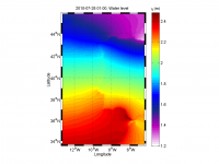
Image:Extrapol_none.png|No extrapolation | Image:Extrapol_none.png|No extrapolation | ||
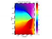
Image:Extrapol_geometric.png|Geometric extrapolation | Image:Extrapol_geometric.png|Geometric extrapolation | ||
Revision as of 13:46, 10 February 2012
Extrapolation is often required when interpolation techniques cannot be used; often when mapping information from one dataset to a grid. Extrapolation methods vary, yielding different results both in quality and in performance. This article proposes a couple of simple extrapolation techniques that use all the information available to extrapolate. The techniques inspire from the weighted average principle.
Contents
Weighted Average
Suppose you have a discrete dataset  , with coordinates
  on a normed space,
  , and want to map the dataset to another dataset,
  , with a new set of coordinates
  . The operation is performed by constructing mapping coefficients
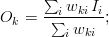
  , also called "weights", and by performing a linear combination of the elements of with the weights, , to compute each element of .
Any method of constructing the weights is valid (as long as  ) and depends on the nature of the mapping. A practical use-case consists in performing an interpolation/extrapolation of the data from to and thus the weights are usually a function of the coordinates and and of the norm of the space. More complex techniques could be used, with also as a function of and its derivatives, but these will not be considered in this text.
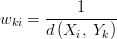
Geometric Weighted Average
The geometric weighted average is the most intuitive approach: it calculates the geometric average of a set of values/points pairs at a given point. The idea is that closer points should have a bigger weight than farther points in the weighted average. In this case, the weight is inversely proportional to the distance:
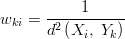
Squared Weighted Average
The same as above, except that the squared norm is used instead of the norm. This gives an even bigger weight to the points that are closer when compared to the geometric average, proportionally to the inverse of the squared distance.
Gaussian Weighted Average
A gaussian weighted average allows to determine characteristic radius of influence,  , where, within that radius, the points of will have a total weight of 68% in the average relative to the other points of . This radius of influence parameter is useful to parameterize the interpolation/extrapolation, by choosing a shorter radius when the interpolating dataset shows greater variability and by choosing a larger radius when the interpolating dataset displays a smooth variability. The isotropic gaussian function is given by:
Failed to parse (unknown error): w_{ki} = \e{\left(-\frac{ d^2\left(X_i,\;Y_k\right)}{\sigma^2}\right)}
- sunflowers are groovy

No extrapolation
Geometric extrapolation
Squared extrapolation
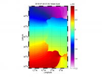
Gaussian extrapolation with
 of the domain characteristic length (average of the width and height)


