Module Waves

Overview

Module Waves is responsible to simulate surface waves in MOHID. It can act as a wave database, reading wave data from files, or it can predict wave parameters through a surface wave generation model which is responsible for computing surface wave properties and its related parameters, therefore communicating directly with the water-air interface module, responsible for all the fluxes between the water column and the atmosphere. The water-air interface module provides wind velocity, direction and shear stresses, receiving from the surface wave module the necessary information to compute water surface rugosity, which can ultimately be used by the turbulence and hydrodynamic module. As surface waves depend and influence water elevations and currents, the wave module also communicates with the hydrodynamic module, providing it with radiation stresses and receiving water depths. Also wave parameters as orbital velocity and excursion are used by the sediment-water interface module to compute bottom shear stresses, which will be used both in hydrodynamics and in sediment transport, controlling erosion and deposition processes.

Deep ocean wave generation model

The surface wave generation model predicts significant wave height and wave period based solely on wind velocity. This approach has applicability mainly in open deep water where wave conditions are not depth and fetch limited.

The Wave Height and Wave Period can be empirically determined as function of wind speed, according to ADIOS model formulations (NOAA, 1994).

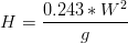$H=\frac{0.243*W^2}g$ equation 1

$T=\frac{8.13*W}g$ equation 2

Where H is Wave Height (m), T is Wave Period (s), W is the wind velocity (m/s) and g the gravity acceleration (m/s²).

Fetch-based wave generation model

The surface wave generation model predicts significant wave height and wave period at the end of generation zone based on fetch, water depth and wind speed and direction. The model is restricted to surface wave generation by local wind and propagation is not considered explicitly. As a consequence, this model can only be applied to areas where wave propagation from the exterior is limited (e.g. ocean swell). Examples of such areas are coastal lagoons, lakes or estuaries with limited wave interaction with the ocean.

Algorithm

In areas where the fetch is not restricted (e.g. open sea), there is a dominant fetch and small changes in wind direction don’t significantly change fetch length or the direction of the generated wave. On the other hand, for wind directions parallel to the shore and mainly for lakes, lagoons or estuaries, a small variation in the wind direction can generate significant changes in the wind’s length of action. In these areas there is not a predominant direction for fetch. In order to calculate the effective fetch it is then necessary to take into account the local morphology of the study area considering several directions, each one with a different weight. Thus, for the same wind direction, a point with more obstacles in the near directions has assigned a smaller fetch than a point with more water length in the same directions. These distances are then used to calculate the effective fetch on each cell, in only 8 cardinal directions. Thus, this calculus is only made once, having each cell 8 values of effective fetch. The result is stored in memory during the entire simulation. During the simulation period, in each time step and in each and every cell, depending on wind direction, the effective fetch is selected from the list of 8 values, and it’s used together with wind speed and water depth to calculate the wave parameters. There are some limitations computing effective fetch when simulating domains with large open boundaries, because there is no information to evaluate fetch distances in the boundaries when wind is blowing from the exterior. Effective fetch is computed considering the highest water level in the simulation domain. This means that when if there are areas that during the simulation become uncovered (e.g. forming a temporary tidal flat island), effective fetch is not adjusted. In those cells, all calculus is switched off until they are flooded again.

Equations

As propagation is not considered, the model does not require any initial conditions and there's no time dependency in the wave parameters evolution. Thus, significant wave height and mean wave period can be computed directly, being only required to provide the necessary input variables: wind speed, water depth and fetch. The equations were adapted from the CE-QUAL-W2 model (Cole, 2003) and were previously developed by Seymour (1977) and Kang et al. (1982).

Failed to parse (unknown error): Hs=\frac{W^2}g0.283\tanh\left[0.53\left(\frac{gH}{W^2}}\right)^{0.75}\right]\tanh\left[\frac{0.0125\left(\frac{gF}{W^2}\right)^{0.42}}{\tanh\left[0.53\left(\frac{gH}{W^2}\right)^{0.75}\right]}\right] equation 3

Failed to parse (unknown error): Ts=\frac{2\pi W}g1.2\tanh\left[0.833\left(\frac{gH}{W^2}}\right)^{0.375}\right]\tanh\left[\frac{0.077\left(\frac{gF}{W^2}\right)^{0.25}}{\tanh\left[0.833\left(\frac{gH}{W^2}\right)^{0.375}\right]}\right] equation 4

Where, H_s is Significant Wave Height, T_s is Significant Wave Period, W is the wind velocity modulus (m/s), H the water depth (m) and F, the fetch distance (m).

These equations predict wave height and wave period at the end of the generation zone, therefore the duration of the wind action it is not accounted for, because it is admitted that the total development of the waves is achieved. The hyperbolic function in eq. 3 and eq. 4 simulates the effects that, for high depths, waves are not influenced by the bottom and is also used to avoid the indefinite increasing of wave height and wave period with increasing fetch. A multiplicative factor for both wave height and period are included in the equations (unitary default value) enabling the calibration of the model results against available waves data.

The broader equation (eq. 5) for effective fetch (F_e) was obtained from Rogala (1997) and Howes (1997):

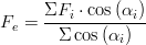$F_e=\frac{\Sigma F_i\cdot\cos\left(\alpha_i\right)}{\Sigma\cos\left(\alpha_i\right)}$ equation 5

Where F_i is the fetch distance (m) in the i direction and α_i = angle (º) between the wind direction and the i direction. For the fetch directions, 3 or 5 distances (eq. 6 and eq. 7 respectively) can be used (dependent on keyword WIND_ROSE_DIRECTIONS - 8 or 16 respectively). This is called the effective modified fetch (Fm):

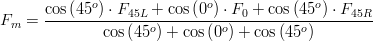$F_m=\frac{\cos\left(45^o\right)\cdot F_{45L}+\cos\left(0^o\right)\cdot F_{0}+\cos\left(45^o\right)\cdot F_{45R}}{\cos\left(45^o\right)+\cos\left(0^o\right)+\cos\left(45^o\right)}$ equation 6

$F_m=\frac{\cos\left(45^o\right)\cdot F_{45L}+\cos\left(22.5^o\right)\cdot F_{22.5R}+\cos\left(0^o\right)\cdot F_{0}+\cos\left(22.5^o\right)\cdot F_{22.5L}+\cos\left(45^o\right)\cdot F_{45R}}{\cos\left(45^o\right)+\cos\left(22.5^o\right)+\cos\left(0^o\right)+\cos\left(22.5^o\right)+\cos\left(45^o\right)}$ equation 7

Where, F_45L and F_22L are the distances to land in the directions 22.5º and 45º left of the wind direction (m); F_45R and F_22R are the distances to land in the directions 22.5º and 45º right of the wind direction (m); and F₀ is distance to land along wind direction (m). The weight given to each distance is based on the cosine function, taking a unitary weight for the wind direction and decreasing weights to angles away from this direction. In order to compute the effective fetch, distances to land need to be computed. As described above the distances can be computed in two different ways: i) in a grid-based method with an algorithm that moves in the grid along the 8 or 16 directions until it finds a land cell or the end of the grid; ii) in a “graphical” method that computes distances between cell centre and land polygons.

Water depth may be computed from 2 methods:

• instant water column in the cell
• average depth in the wind direction

The first method uses the water column in every instant to compute wave height and wave period

The second method in every instant checks the wind direction and gets the average depth in wind direction (computed in construction phase from bathymetry). In this case average depths are computed similarly to Fetch with weighting.

Wave orbital velocity and excursion

Linear wave theory is generally applied to determine the near-bed velocities. In case of symmetrical (sinusoidal) small-amplitude waves in relatively deep waters this theory yields good results. When waves approach shallower waters, the waves will be distorted leading to asymmetrical wave profiles and higher order wave theories are necessary to determine the near-bed velocities. In this model only linear wave theory is considered, therefore applying it, the peak value of the orbital excursion (Aδ) and velocity (Uδ) at the edge of the wave boundary layer can be expressed as:

Insert equation

User manual

Main options

In this chapter it is briefly described how to use Module Waves. The different options provided by the module can be defined through an input data file, similarly to other modules in MOHID. In order to couple this module with the rest of the model simulation, it has to be activated in the Module Model input data file, by defining the following keyword:

WAVES                                     : 1

ModuleWaves can be used as a database, reading the solution for the different parameters (radiation stresses, significant wave height, mean wave period and mean wave direction) from a file, or it can be used to compute wave parameters based on external information. Depending on the options chosen, ModuleWaves might be dependent on the activation of other modules, namely the Atmosphere and InterfaceWaterAir modules, which provide wind information. In order to use the wave module so that it influences hydrodynamics (water level and currents), the user must activate the radiation stress options and activate in the Hydrodynamic input data file the following keyword:

WAVE_STRESS                           : 1

To use Module Waves so that the waves effect contributes to the calculation of bottom shear stress it is necessary to turn on the following keyword and block in InterfaceSedimentWater data file:

WAVETENSION                       : 1

<begin_waverugosity>
INITIALIZATION_METHOD        : CONSTANT
FILE_IN_TIME                 : NONE 
DEFAULTVALUE                 : 9e-3
REMAIN_CONSTANT              : 0 
<end_waverugosity>

This will also enable to consider waves influence on resuspension and deposition of particulate matter in the water-sediment interface.

Keywords

Keyword                   : Data Type         Default     !Comment

RADIATION_TENSION_X       : logical            false        !Connect/Disconnect waves radiation tension in X direction
RADIATION_TENSION_Y       : logical            false        !Connect/Disconnect waves radiation tension in Y direction
WAVE_HEIGHT               : logical             true        !Connect/Disconnect waves height 
WAVE_PERIOD               : logical             true        !Connect/Disconnect waves period
WAVE_DIRECTION            : logical             true        !Connect/Disconnect waves direction
WAVEGEN_TYPE              : integer              0          !Method for computing wave generation (wave height and period)
                                                             ! 0 - deep areas (wind velocity dependent); 
                                                             ! 1 - shallow "closed" areas (wind velocity and direction, fetch and depth dependent)
DISTANCE_TO_LAND_METHOD   : integer              0          !Method for computing fetch distances to land (read if WAVEGEN_TYPE : 1)
                                                             ! 0 - grid based method (limited in nested domains)
                                                             ! 1 - graphical method using distances to land poligons (need the polygon block)
WINDROSE_DIRECTIONS       :  8/16                8          !Number of directions to compute distances to land (read if WAVEGEN_TYPE : 1)
WAVE_HEIGHT_PARAMETER     :  real                1.         !multipling factor for wave height - calibration  (read if WAVEGEN_TYPE : 1)
WAVE_PERIOD_PARAMETER     :  real                1.         !multipling factor for wave period - calibration  (read if WAVEGEN_TYPE : 1)
DEPTH_METHOD              : integer              0          !Method for computing fetch depth  (read if WAVEGEN_TYPE : 1)
                                                             ! 0 - local cell water column
                                                             ! 1 - average depth in the wind direction
                                                             ! 2 - user defined value (constant for sensibility tests)
MEAN_SEA_LEVEL            : real                 0.         !Mean sea level above bathimetry for DEPTH_METHOD : 2 (average bathymetry + MSL)
DEPTH_VALUE               : real             AllmostZero    !Depth defined by user for DEPTH_METHOD : 3
OUTPUT_FETCH_DISTANCES    : logical            .false.      !Output fetch distances in each direction (grid data) (read if WAVEGEN_TYPE : 1)
OUTPUT_FETCH_DEPTHS       : logical            .false.      !Output fetch depths in each direction (grid data) (read if WAVEGEN_TYPE : 1 )

Poligon block for DISTANCE_TO_LAND_METHOD : 1
<begin_landareafiles>
  Polygon1.xy
  Poligon2.xy
   ...
<end_landareafiles>

<begin_[property]>
 NAME                      : wave height/ wave period / ... 

 see Module FillMatrix for more options

<end_[property]>

Input data file

In a simulation, it is possible to choose between the calculation of wave height and wave period as described in deep ocean equations based on wind velocity (simpler) or as fetch and depth dependent. This is made by a keyword named [WAVEGEN_TYPE] (keyword = 0 and the method is the simpler and keyword = 1 stands for the fetch method, by default the value is 0 (zero)).

Fetch based

If using the fetch based model, the working scheme of the model is very simple: in the constructing phase of MOHID, the distances to land are calculated for all water cells in the 8 or 16 cardinal directions defined by the keyword [WINDROSE_DIRECTIONS].

The distances to land can be computed with two different methods, distinguishing them with the keyword [DISTANCE_TO_LAND_METHOD]. If this keyword equals zero, the distances to land are computed along the grid, incrementing half cell size in each cycle step, until land or end of grid is encountered. If the keyword equals one, distances are computed performing tangents to the points and intersecting them with polygons (Land Areas) segments. The first method can not be used with nested models (if grid ends before directions reaches land).

Fetch distances are only calculated once in the simulation (in the MOHID construction phase).

Wind velocity based example

OUTPUT_TIME              : 0 86400

RADIATION_TENSION_X      : 0
RADIATION_TENSION_Y      : 0
WAVE_PERIOD              : 1
WAVE_HEIGHT              : 1
WAVE_DIRECTION           : 1

WAVEGEN_TYPE             : 0
  
<begin_waveperiod>
INITIALIZATION_METHOD    : CONSTANT
DEFAULTVALUE             : 12.
REMAIN_CONSTANT          : 0
OUTPUT_HDF               : 1
TIME_SERIE               : 1
<end_waveperiod>
 
<begin_waveheight>
INITIALIZATION_METHOD    : CONSTANT
DEFAULTVALUE             : 0.1
REMAIN_CONSTANT          : 0
OUTPUT_HDF               : 1
TIME_SERIE               : 1
<end_waveheight>

<begin_wavedirection>
INITIALIZATION_METHOD    : CONSTANT
DEFAULTVALUE             : 0.
REMAIN_CONSTANT          : 0
OUTPUT_HDF               : 1
TIME_SERIE               : 1
<end_wavedirection>

Fetch based example

OUTPUT_TIME              : 0 86400

RADIATION_TENSION_X      : 0
RADIATION_TENSION_Y      : 0
WAVE_PERIOD              : 1
WAVE_HEIGHT              : 1
WAVE_DIRECTION           : 1

WAVEGEN_TYPE             : 1
                  
WINDROSE_DIRECTIONS      : 16
WAVE_HEIGHT_PARAMETER    : 1.     
WAVE_PERIOD_PARAMETER    : 1.  

DEPTH_METHOD             : 1
MEAN_SEA_LEVEL           : 2.08
 
OUTPUT_FETCH_DISTANCES   : 1
OUTPUT_FETCH_DEPTHS      : 1


<begin_waveperiod>
INITIALIZATION_METHOD    : CONSTANT
DEFAULTVALUE             : 12.
REMAIN_CONSTANT          : 0
OUTPUT_HDF               : 1
TIME_SERIE               : 1
<end_waveperiod>
 
<begin_waveheight>
INITIALIZATION_METHOD    : CONSTANT
DEFAULTVALUE             : 0.1
REMAIN_CONSTANT          : 0
OUTPUT_HDF               : 1
TIME_SERIE               : 1
<end_waveheight>

<begin_wavedirection>
INITIALIZATION_METHOD    : CONSTANT
DEFAULTVALUE             : 0.
REMAIN_CONSTANT          : 0
OUTPUT_HDF               : 1
TIME_SERIE               : 1
<end_wavedirection>

SWAN based example

This example MOHID input data files shows how to read wave forcing from an hdf5, generated from the results of a wave model, one such as SWAN. Go check out the SWAN wiki to configure and run the SWAN for your domain...

Hydrodynamic_x.dat
 
WAVE_STRESS             : 1

InterfaceSedimentWater_x.dat
 
<begin_waverugosity>
FILE_IN_TIME            : NONE
REMAIN_CONSTANT         : 0
OUTPUT_HDF              : 1
TIME_SERIE              : 0
DEFAULTVALUE            : 0.0025
<end_waverugosity>
 
WAVETENSION : 1

Waves_x.dat
 
WAVE_PERIOD             : 1
WAVE_DIRECTION          : 1
WAVE_HEIGHT             : 1
RADIATION_TENSION_X     : 1
RADIATION_TENSION_Y     : 1
 
<begin_waveheight>
NAME                    : significant wave height
UNITS                   : m
DESCRIPTION             : wave height variable
INITIALIZATION_METHOD   : HDF
FILE_IN_TIME            : HDF
FILENAME                : Waves.hdf5
DEFAULTVALUE            : 0.0
OUTPUT_HDF              : 1
<end_waveheight>
 
<begin_wavedirection>
NAME                    : mean wave direction
UNITS                   : º
DESCRIPTION             : mean wave direction
INITIALIZATION_METHOD   : HDF
FILE_IN_TIME            : HDF
FILENAME                : Waves.hdf5
DEFAULTVALUE            : 0.0
OUTPUT_HDF              : 1
<end_wavedirection>
 
<begin_waveperiod>
NAME                    : mean wave period
UNITS                   : s
DESCRIPTION             : mean wave period WW3
INITIALIZATION_METHOD   : HDF
FILE_IN_TIME            : HDF
FILENAME                : Waves.hdf5
DEFAULTVALUE            : 0.0
OUTPUT_HDF              : 1
<end_waveperiod>
 
<begin_radiationstress_x>
NAME                    : wave stress X
UNITS                   : Pa
DESCRIPTION             : /wave stress X
INITIALIZATION_METHOD   : HDF
FILE_IN_TIME            : HDF
FILENAME                : Waves.hdf5
DEFAULTVALUE            : 0.0
OUTPUT_HDF              : 1
<end_radiationstress_x>
 
<begin_radiationstress_y>
NAME                    : wave stress Y
UNITS                   : Pa
DESCRIPTION             : /wave stress Y
INITIALIZATION_METHOD   : HDF
FILE_IN_TIME            : HDF
FILENAME                : Waves.hdf5
DEFAULTVALUE            : 0.0
OUTPUT_HDF              : 1
<end_radiationstress_y>

References

• Braunschweig F, Leitao PC, Fernandes L, Pina P, Neves RJJ. The object oriented design of the integrated Water Modelling System. Developments in Water Science. 2004;55:1079-1090. Available at: http://dx.doi.org/10.1016/S0167-5648(04)80126-6.

• Cole, T.M. and S.A. Wells, 2003. CE-QUAL-W2: A two-dimensional, laterally averaged, Hydrodynamic and Water Quality Model, Version 3.2. Instruction Report EL-03-1, US Army Engineering and Research Development Center, Vicksburg, MS.

• Howes, 1997. British Columbia Estuary mapping Systems – Appendix A: Wave Exposure Calculation. Ministry of Sustainable Resource Management, British Columbia U.S.A.

• Kang, S.W., Sheng, J.P. and Lick, W., 1982. Wave Action and Bottom Shear Stress in Lake Eire. Journal of Great Lake Research, 8(3): 482-494.

• NOAA (1994) - ADIOSTM (Automated Data Inquiry for Oil Spills) user’s manual. Seattle: Hazardous Materials Response and Assessment Division, NOAA. Prepared for the U.S. Coast Guard Research and Development Center, Groton Connecticut, 50 pp.

• Rogala, J.T., 1997. Estimating Fetch for Navigation Pools in the Upper Mississippi River Using a Geographic Information System. United States Geological Survey -Project Status Report 97-08 .

• Seymour, R.J., 1977. Estimating Wave Generation in Restricted Fetches. J. ASME WW2, May 1977 pp251-263.