SmoothBatimNesting
From MohidWiki

This program creates a new sub-model bathimetry to allow a smooth transition in the boundary between the coarser model and the high resolution model. See also SmoothBatimCoefs.
Quick start
- Create the father and son bathymetries (you may use Mohid GIS).
- Create the SmoothCoeficients griddata file (you may use SmoothBatimCoefs).
- Create and edit the options SmoothBatimNesting.dat file and save it in the same path as the executable.
- Run the executable.
Options file
Here's what the options file SmoothBatimNesting.dat looks like:
FATHER_BATIM                : ..\..\WestIberiaTide\GridData.dat
SON_BATIM                   : ..\GridData_2.dat
SMOOTH_COEF                 : SmoothCoef.dat
NEW_SON_BATIM               : SmoothData.dat
Smoothing algorithm
Let it be  , as an element of the father, the son and the interpolated bathymetries discrete fields. Let it be
  as the respective index mapping function. Let it be
  , a continuous map, so that
  . Let
. Let  define the work domain of
  . In particular,
  verifies
  . The son grid is the same as the interpolated grid, meaning
  . However, the father field is completely independent from the other fields, meaning that
  . The smoothing algorithm is a simple linear interpolation of the father and son fields:
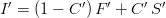
where the smoothing coefficient is given by ![C^\prime: \mathbb{R}^2 \longrightarrow \left[0\;1\right]](/images/math/3/6/9/369d5cf0d68b7852eb9f308576a33a4d.png) . Thus, the smoothing coefficient gridded counterpart
. Thus, the smoothing coefficient gridded counterpart  is defined; and its index mapping function
  is equal to the son's; meaning
  . Let us define the grid
  such that
  and
and  . Thus the smoothing coefficient needs can be defined in
  . Concretely speaking,
 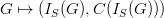 is the smoothing coefficient's Grid Data file described above, thus it leaves to the modeller the choice of the smoothing coefficient field.
Implementation
Let us define a collection of four-vertices polygons taken from the father grid:
where  is the subdomain defined by the vertices of
  .
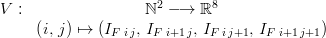
Let us define an auxiliary grid of the son grid given by:
.
Let us define an auxiliary grid of the son grid given by:
 .
.
Let us define a new mapping into a subset of  's image:
- \
 .
.
Here's the implemented smoothing algorithm:
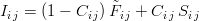 .
.